NOAA RAP Dataset
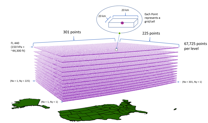
The NOAA RAP data is an open-source hourly updated collection and model forecast system. It obtains atmospheric data through a combination of sources including commercial aircraft, weather balloons, radar, and satellites. Below is a visualization of a grid that depicts how GRIB2 grids cover the airspace over CONUS. Each cell represents a 20 km by 20 km area for a particular flight level.
Essentially, the RAP GRIB2 data contains weather information and details of a three-dimensional grid within the United States’ airspace. By providing environmental situational awareness, in hourly increments, and various atmospheric condition data for a 20-km spatial resolution grids, at fixed interval pressure levels (100 hPa – 1,000 hPa) our team was able to utilize the RAP dataset for short-range weather forecasting, specifically focusing on the presence of the Ice Supersaturated Regions within CONUS (the contiguous/continental United States).
ADS-B Tracking Data
Our second data set, ADS-B data is utilized by air traffic control to display an aircraft’s altitude, velocity, position, and other surveillance data. This dataset has been collected by members of the aviation community who use feeders to receive the broadcasting data from aircrafts. This data is then supplied back through the ADSBExhange through application programming interfaces (APIs)
This dataset provides information regarding altitiude, airspeed, and location of thorusands of aicrafts a a time. ADS-B data was used to overlay onto ISSR hotspots identified. It helped our team idenitfy where and when aircrafts are most likely to fly through ISSRs and form Aircraft-Induced Clouds. For the purpose of our analysis, we utilized one day's worth of ADS-B data (June 6, 2020) assuming that this day represents a tyupical day of flight operations.
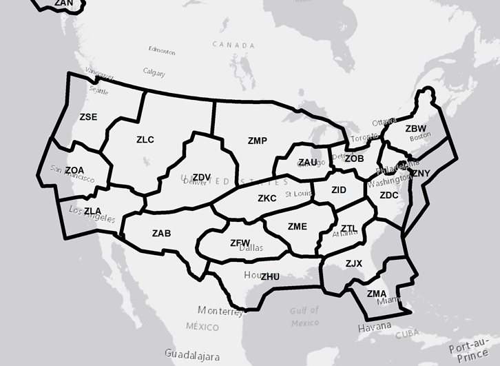
ARTCC Boundary Data
Our third data set, the ARTCC boundary dataset, is a collection of latitude/longitude points along the boundaries of each ARTCC region. These boundaries divide the regions of CONUS where each Air Traffic COntrol Center is responsible for controlling flight traffic. This dataset allowed us to divide the CONUS into regions and identify which regions had the most air traffic, which are most likely to experience ISSRs, and which are most susceptible to AICs formation.